When Being Right Isn't Enough

The Gambler Who Knew the Odds

In the winter of 1961, a skinny math professor named Edward Thorp walked into a casino in Reno, Nevada, with ten thousand dollars that wasn't his. The money belonged to two wealthy gamblers — Emmanuel Kimmel and Eddie Hand — who'd bankrolled Thorp after reading about his blackjack research in the Washington Post. Thorp had done something no one had done before: he'd proven, mathematically, that a card counter could gain a genuine edge over the house. The casinos weren't random. They were beatable.1

But here's the thing almost nobody talks about: Thorp already knew how to win. The harder problem — the problem that would consume the next fifty years of his career and make him hundreds of millions of dollars — was figuring out how much to bet.

Picture this. You've cracked the code. You know the deck is rich in tens and aces, and the math says you have a 2% edge on the next hand. So you shove all your chips in, right? You have an edge. You're right.

And this is where most smart people go broke.

Thorp didn't figure this out alone. A year earlier, at MIT, he'd knocked on the office door of Claude Shannon — the father of information theory, arguably the most brilliant scientist in America — to discuss his blackjack research. Shannon was intrigued. The two men spent hours at Shannon's home in Winchester, Massachusetts, a sprawling Victorian crammed with unicycles, flame-throwing trumpets, and homemade robots. Amid this chaos, Shannon pointed Thorp to a 1956 paper by a Bell Labs physicist named John Larry Kelly Jr.2

Kelly's paper had nothing to do with gambling. It was about a technical problem in information theory: how to maximize the growth rate of wealth when you receive noisy signals over a telephone line.3 But its implications were explosive. Kelly had derived a formula — elegant, simple, and deeply counterintuitive — that told you exactly how much to bet when you have an edge.

And the formula's most important lesson wasn't about what to do. It was about what not to do.

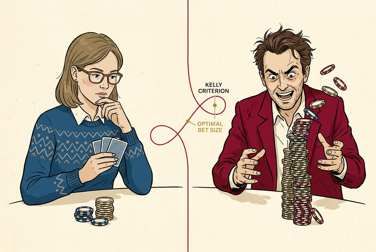
The Gambler Who Bets Too Much

Let's start with a thought experiment. I'm going to offer you a bet that's absurdly in your favor. A coin flip, but rigged: 60% chance you win, 40% chance you lose. When you win, you double your bet. When you lose, you lose your bet. You start with $1,000, and you're going to flip this coin 100 times.

What fraction of your bankroll should you bet each time?

Your expected value is positive on every single flip. The arithmetic says bet big. Bet everything. After all, each bet has a positive expected return of 20 cents on the dollar. The more you bet, the more you expect to make.

Try it and see what happens.

If you just ran that simulation — and you should, because the feeling matters more than the explanation — you noticed something strange. Betting 100% of your bankroll every time, which maximizes your expected value on each individual flip, almost certainly leaves you broke. Not unlucky-broke. Mathematically-certainly broke. One loss wipes you out, and in 100 flips, you will lose at least once.

Okay, 100% is obviously dumb. But what about 80%? Or 50%? This is where it gets weird. Even betting 50% of your bankroll — with a 60% chance of winning each flip — will probably ruin you over 100 rounds. You'll have spectacular runs where you're up 10x, followed by a string of losses that erases almost everything.

The problem is that your bankroll doesn't grow by addition. It grows by multiplication. Each bet multiplies your wealth by some factor. And when you're multiplying, a different kind of average matters.

Two Averages Walk Into a Bar

Here's the mathematical heart of it.

Say you bet 50% of your $1,000. You win (60% chance), and now you have $1,500. You lose (40% chance), and you have $500. Your expected wealth after one round is:

A 10% expected gain. Beautiful. But now play two rounds. If you win then lose (or lose then win), you have:

You won exactly half your bets with a positive-expected-value wager, and you lost money. The arithmetic mean — the expected value — says you're making 10% per round. But the geometric mean — the thing that actually determines your long-run compound growth — says something different.

For our 60/40 coin at even odds, you can take the derivative, set it to zero, and get the Kelly fraction:

The Kelly Formula

Let's write it more generally. You have a bet where you win with probability p, and when you win, you get b dollars for every dollar wagered (and lose your dollar when you lose). The Kelly fraction is:

f*

Optimal fraction of wealth to bet

p

Probability of winning

b

Net odds — profit per dollar wagered on a win

Play with that calculator. Notice something? Even Thorp's blackjack edge — maybe a 2% advantage in the best situations — calls for betting only about 2–4% of your bankroll on any given hand. Not 10%. Not 25%. The formula is conservative in a way that feels almost timid to people who know they have an edge.

That's the point.

Why Geometric Means Rule the World

Kelly's formula works because of a mathematical fact about repeated multiplication that most people — including most very smart people — don't intuitively grasp.

When you play a game repeatedly, reinvesting your winnings each time, your long-run wealth isn't determined by the average outcome. It's determined by the typical outcome. And in a multiplicative world, those are very different things.

This gap between the average and the typical — between the arithmetic mean and the geometric mean — is one of the most important ideas in all of applied mathematics. It shows up in evolutionary biology, in population genetics, and in every investment decision you've ever made.6

Fractional Kelly: The Real World

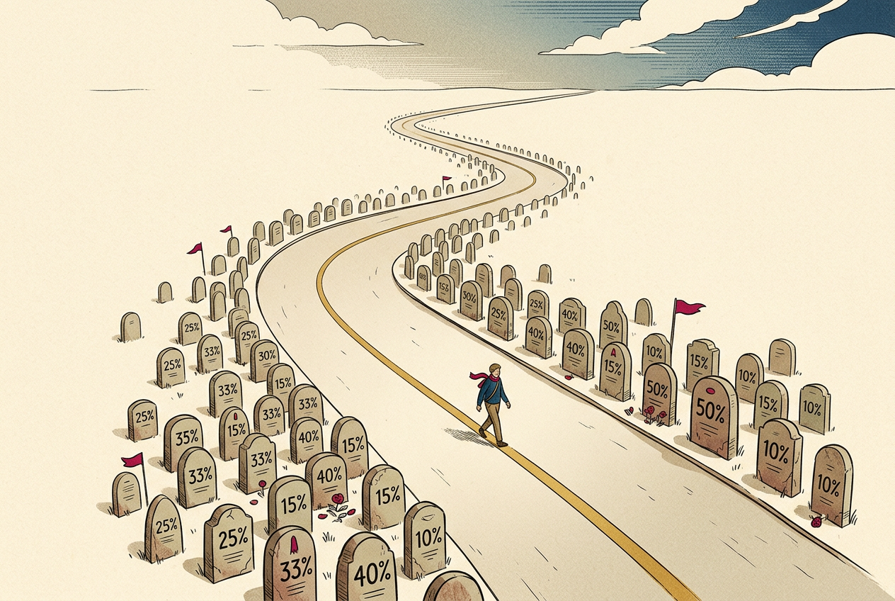
Now here's where I have to be honest with you about Kelly's limitations, because the formula in its pure form assumes you know things you almost never know.

It assumes you know your exact edge. In blackjack, Thorp could estimate it — the math is clean, the deck is finite. But in the stock market? In a startup investment? In your career bet on a new industry? You think you have an edge. You might be right. But you're not sure, and if you overestimate your edge, the Kelly formula tells you to bet too much.

This maps to a broader life principle. When you have an edge — in a career move, an investment, a business decision — the biggest danger isn't betting too small. It's betting too big. The cost of underbetting is linear: you grow a bit slower. The cost of overbetting is catastrophic: you can lose everything.

The Bet You're Always Making

Here's what makes the Kelly criterion more than a gambling trick or an investing technique. It's a model for every decision where you reinvest the consequences.

You're choosing between two job offers. One is safe: steady salary, clear trajectory, modest upside. The other is a startup: it could make you rich, it could waste three years of your life. Kelly doesn't say take the safe job. And it doesn't say take the risky one. It says: how much of your life are you betting?

If you're 25 with no dependents and a safety net, you can afford a larger Kelly fraction. The startup is a reasonable bet. If you're 45 with a mortgage and two kids in private school, the same bet might be catastrophic overbetting — not because the expected value is different, but because the consequences of ruin are different.

Edward Thorp understood this at a blackjack table in 1961. He spent the next six decades proving it, first in casinos, then on Wall Street — where his hedge fund, Princeton Newport Partners, returned nearly 20% annualized over two decades8 — then as one of the most successful investors in American history.7 And the deepest lesson he took from Kelly's formula wasn't about maximizing returns. It was about survival.

The Kelly criterion respects this asymmetry. It's the mathematics of not going broke — which turns out to be the most important mathematics of all.